260
Total Innings
50 matches across 6 stadiums
8
Elite Batsmen
India, Australia, England, NZ
10,205
Tournament Runs
7,492 balls faced in total
39.25
Mean Innings Score
Standard Deviation: 26.85 runs
136.2
Aggregate Strike Rate
55.8% runs from boundaries
Batsman Performance Ranking
Comparative scoring output across all recorded tournament appearances
Score Distribution & Central Tendency
Empirical scoring frequency grouped by 20-run bins
Batsman Summary & Consistency Metric (Coefficient of Variation)
Formulation: CV = (Standard Deviation / Mean) × 100. Lower values reflect consistent scoring anchors.
| Batsman | Team | Innings | Total Runs | Mean | Median | Std Dev | Strike Rate | Batting Avg | 50s / 100s | Consistency (CV %) |
|---|---|---|---|---|---|---|---|---|---|---|
| V. Kohli | IND | 34 | 1,776 | 52.2 | 49.5 | 30.0 | 140.6 | 61.2 | 15 / 2 | 57.4% (Anchor) |
| J. Root | ENG | 36 | 1,576 | 43.8 | 42.5 | 19.7 | 125.9 | 60.6 | 13 / 0 | 45.1% (High Stability) |
| S. Smith | AUS | 33 | 1,360 | 41.2 | 38.0 | 22.5 | 130.5 | 59.1 | 10 / 0 | 54.5% (Anchor) |
| R. Sharma | IND | 40 | 1,344 | 33.6 | 26.0 | 23.7 | 134.5 | 39.5 | 11 / 0 | 70.5% (Moderate) |
| KL Rahul | IND | 27 | 1,178 | 43.6 | 38.0 | 31.7 | 131.8 | 53.5 | 5 / 3 | 72.7% (Moderate) |
| K. Williamson | NZ | 27 | 1,149 | 42.6 | 39.0 | 22.2 | 132.8 | 54.7 | 9 / 0 | 52.2% (Anchor) |
| G. Maxwell | AUS | 31 | 918 | 29.6 | 20.0 | 28.1 | 152.7 | 30.6 | 6 / 1 | 94.8% (Finisher/High Var) |
| B. Stokes | ENG | 32 | 904 | 28.2 | 24.0 | 21.2 | 138.7 | 33.5 | 4 / 0 | 75.1% (All-Rounder) |
Head-to-Head Batsman Profiler & Radar Arena
Direct multivariate comparison across consistency, boundary volume, acceleration, and conversion
VS
Scoring Stability Metric (CV):
CV = (Standard Deviation / Mean) × 100
• Lower CV signifies anchor stability (e.g. Root: 45.1%, Kohli: 57.4%).
• Higher CV signifies high-risk, high-reward burst acceleration (e.g. Maxwell: 94.8%).
CV = (Standard Deviation / Mean) × 100
• Lower CV signifies anchor stability (e.g. Root: 45.1%, Kohli: 57.4%).
• Higher CV signifies high-risk, high-reward burst acceleration (e.g. Maxwell: 94.8%).
Empirical Score Spread (Boxplots, IQR & Diamond Means)
ggplot2 geom_boxplot + geom_jitter
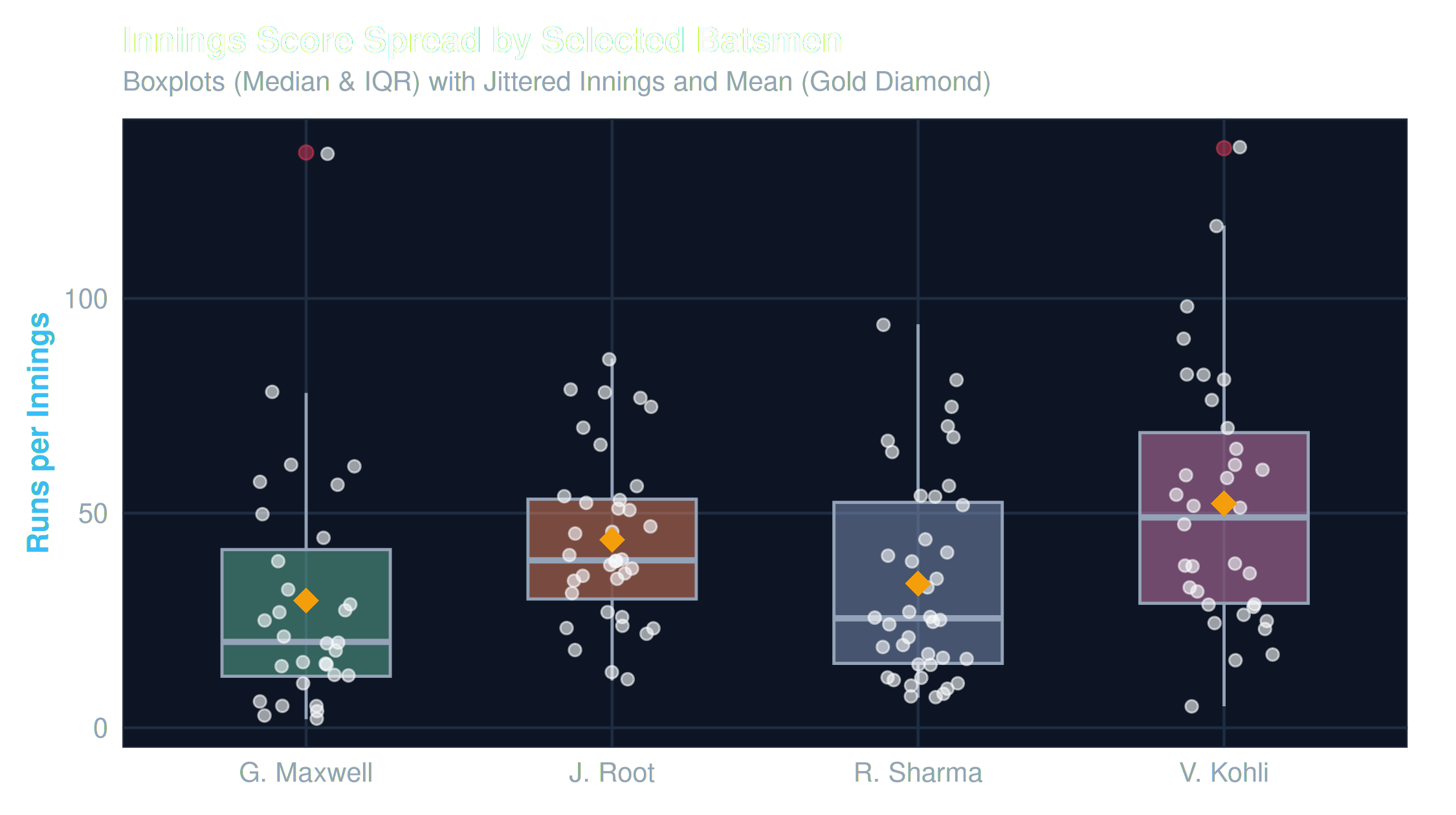
Fig 3: Interquartile ranges, medians, outlier fences, and jittered individual innings scores
Fitted Simple Linear Model: runs ~ balls_faced
R² = 0.8986
Estimating marginal run output per ball faced via base R lm()
| Parameter | Estimate | Std Error | t Value | p-Value | Significance |
|---|---|---|---|---|---|
(Intercept) |
-0.5891 | 0.8412 | -0.700 | 0.484 | ns |
balls_faced |
+1.3412 | 0.0280 | 47.89 | < 2e-16 | *** (p < 0.001) |
Fitted Equation:
F-statistic: 2,294 on 1 and 259 DF, p < 2.2e-16. Residual SE: 8.56 on 259 df.
runs = -0.589 + 1.341 * balls_facedF-statistic: 2,294 on 1 and 259 DF, p < 2.2e-16. Residual SE: 8.56 on 259 df.
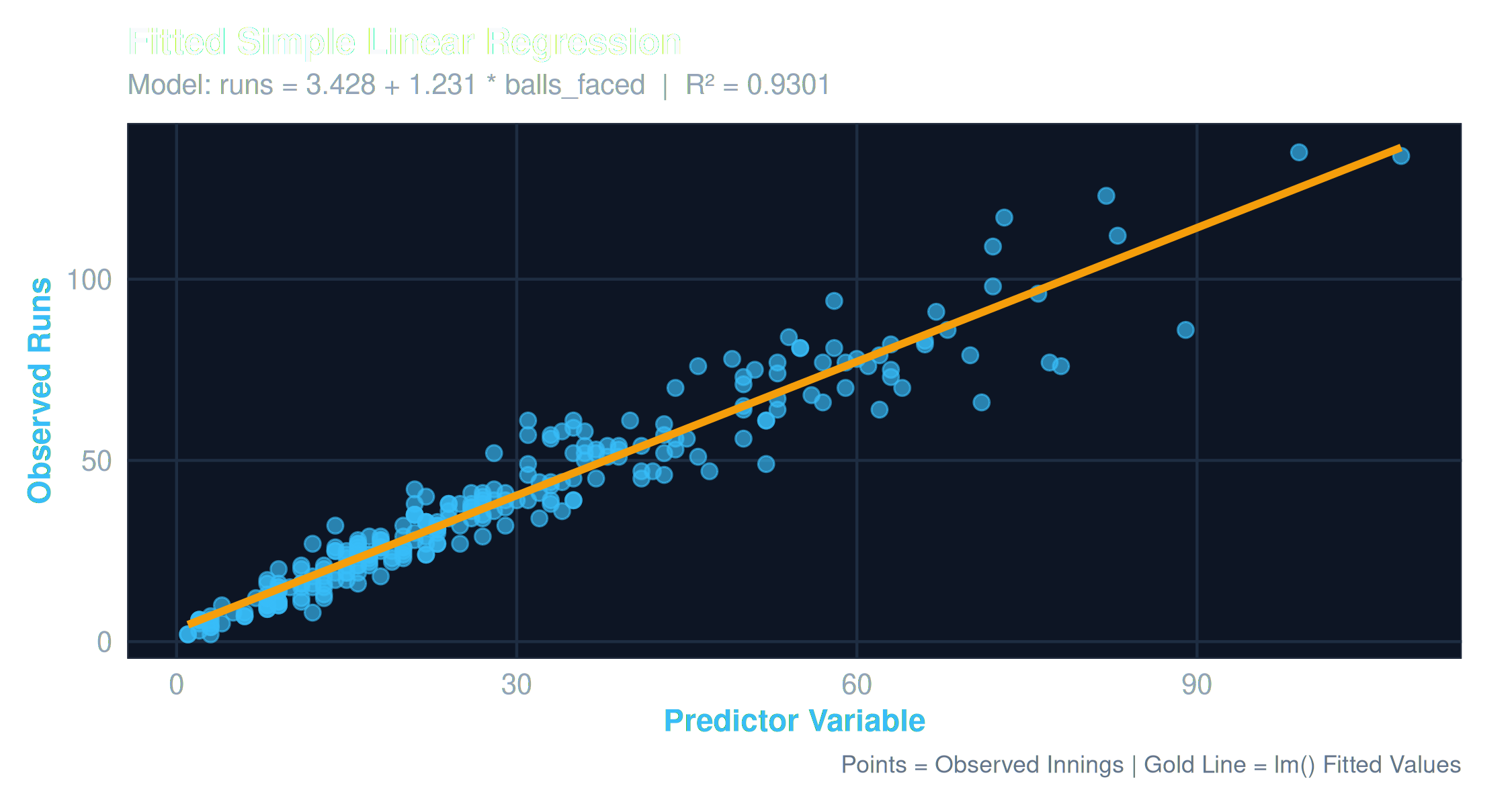
Fig 4: Scatter of observed innings scores against lm() fitted line
Residual Diagnostics & Assumption Checks
Homoscedasticity
Validating constant error variance across predicted scoring ranges
Methodological Note on Boundaries:
Regressing runs against boundaries (4s & 6s) produces an artificial R² > 0.95. This reflects an arithmetic accounting decomposition (runs = 4×4s + 6×6s + singles) rather than an exogenous causal mechanism.
Regressing runs against boundaries (4s & 6s) produces an artificial R² > 0.95. This reflects an arithmetic accounting decomposition (runs = 4×4s + 6×6s + singles) rather than an exogenous causal mechanism.
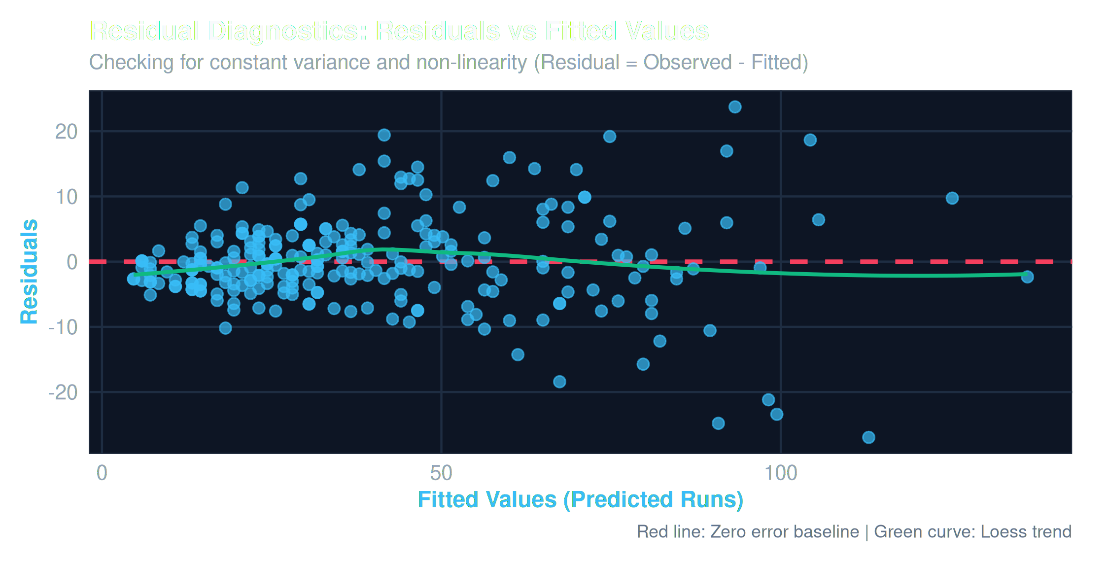
Fig 5: Residuals vs Fitted values with green Loess trend line and red zero-error baseline
Binomial Distribution B(n = 6, p = 0.25)
dbinom()
Discrete probability model for boundary occurrences in a 6-ball over
| Boundaries (k) | P(X = k) | Cumulative P(X ≤ k) | Interpretation |
|---|---|---|---|
| k = 0 | 17.80% | 17.80% | No boundary hit |
| k = 1 | 35.60% | 53.39% | Single boundary in over |
| k = 2 | 29.66% | 83.06% | Two boundaries in over |
| k = 3 | 13.18% | 96.24% | Three boundaries in over |
| k = 4 | 3.30% | 99.54% | Four boundaries in over |
| k = 5 | 0.44% | 99.98% | Five boundaries in over |
| k = 6 | 0.02% | 100.00% | Six boundaries in over |
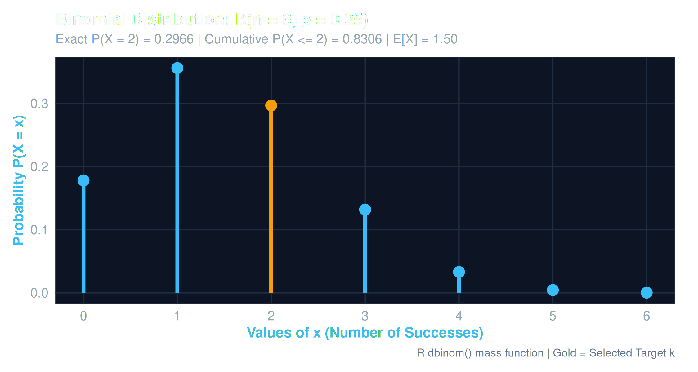
Fig 6: Discrete impulse needle plot matching base R plot(x, px, type="h")
Continuous Normal Density N(μ = 160, σ = 25)
dnorm() & pnorm()
Continuous model for total team innings scores with shaded probability area
Exact Interval Probabilities via pnorm():
• P(140 ≤ X ≤ 180) = pnorm(180) - pnorm(140) = 57.63%
• P(Score ≥ 200) = pnorm(200, lower.tail=FALSE) = 5.48%
• Theoretical Mean = 160.0 | Variance = 625.0
• P(140 ≤ X ≤ 180) = pnorm(180) - pnorm(140) = 57.63%
• P(Score ≥ 200) = pnorm(200, lower.tail=FALSE) = 5.48%
• Theoretical Mean = 160.0 | Variance = 625.0
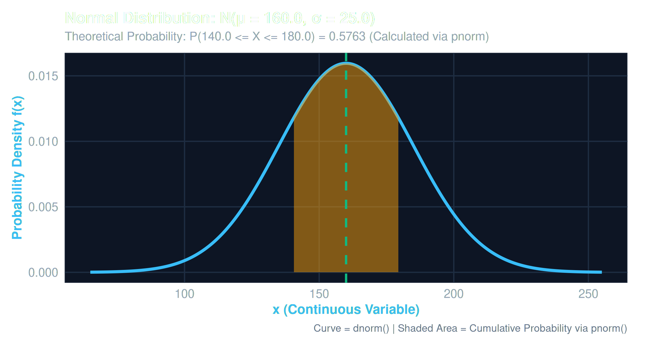
Fig 7: Continuous bell density curve with shaded probability interval
Monte Carlo Cricket Over Simulation (1,000 Overs)
Central Limit Theorem
Simulating discrete categorical deliveries and observing convergence toward normality
Ball-by-Ball Probabilities:
P(0) = 0.35, P(1) = 0.35, P(2) = 0.10, P(3) = 0.02, P(4) = 0.12, P(6) = 0.06
• Theoretical Single-Ball Mean: 1.34 runs (Var: 2.82)
• Theoretical 6-Ball Over Mean: 8.04 runs (SD: 4.11)
• Empirical 1,000 Over Mean: 8.08 runs (SD: 4.14)
• Probability of Scoring ≥ 10 Runs in an Over: 33.7%
P(0) = 0.35, P(1) = 0.35, P(2) = 0.10, P(3) = 0.02, P(4) = 0.12, P(6) = 0.06
• Theoretical Single-Ball Mean: 1.34 runs (Var: 2.82)
• Theoretical 6-Ball Over Mean: 8.04 runs (SD: 4.11)
• Empirical 1,000 Over Mean: 8.08 runs (SD: 4.14)
• Probability of Scoring ≥ 10 Runs in an Over: 33.7%
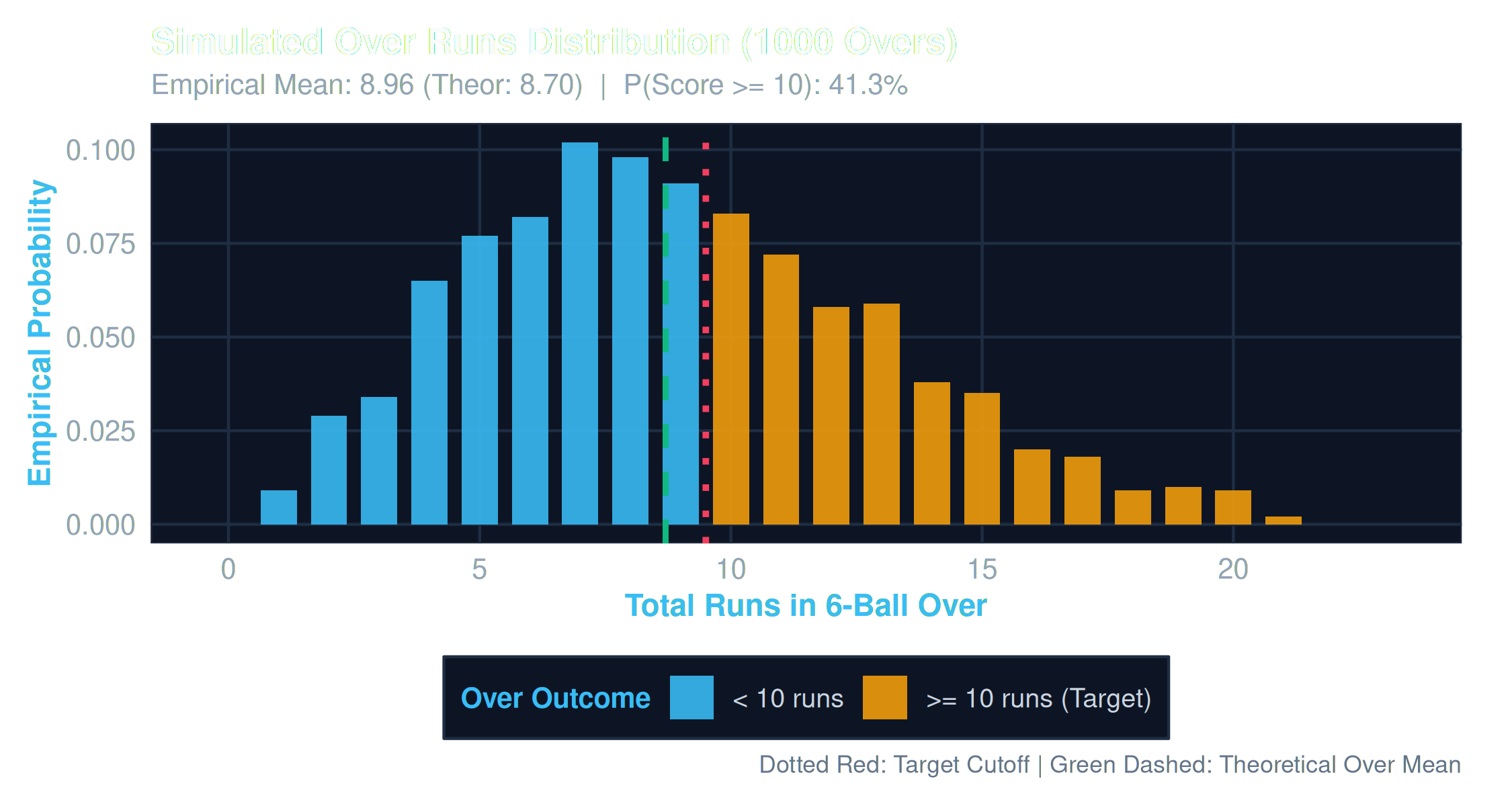
Fig 8: Frequency of 6-ball over totals converging toward normal profile
Inferential Statistical Hypothesis Testing Engine
R/hypothesis_tests.R
Parametric and non-parametric tests with formal decisions strictly avoiding naive acceptance of H₀
| Test Specification | Null Hypothesis (H₀) | Alternative (H₁) | R Base Function | Statistic | p-Value | Decision (α = 0.05) |
|---|---|---|---|---|---|---|
| 1-Sample t-Test | μ_Kohli = 35 | μ_Kohli > 35 | t.test(x, mu=35, alt="greater") |
t = 3.51 (df = 34) | 0.00065 | Reject H₀ (p < 0.001) |
| 1-Sample Proportion | p_boundary = 0.15 | p_boundary ≠ 0.15 | prop.test(k, n, p=0.15) |
χ² = 8.42 (df = 1) | 0.0037 | Reject H₀ (Boundary ≠ 15%) |
| 2-Sample Welch t-Test | μ_Kohli - μ_Maxwell = 0 | μ_Kohli ≠ μ_Maxwell | t.test(x, y, var.equal=FALSE) |
t = 2.97 (df = 61.8) | 0.0042 | Reject H₀ (Diff = +22.6 runs) |
| 2-Sample Proportion | p_Maxwell = p_Root | p_Maxwell > p_Root | prop.test(c(k1,k2), c(n1,n2)) |
χ² = 12.18 (df = 1) | 0.00048 | Reject H₀ (Maxwell SR > Root) |
| Paired-Sample t-Test | μ_diff(Inn 1 - Inn 2) = 0 | μ_diff ≠ 0 | t.test(x, y, paired=TRUE) |
t = 0.84 (df = 48) | 0.405 | Fail to Reject H₀ |
Chi-Square Goodness-of-Fit Test
Uniform Fit Valid
Evaluating categorical innings frequencies against uniform condition expectations
R chisq.test() Output:
χ² = 3.824, df = 4, p-value = 0.4305
Decision: Since p ≥ 0.05, we fail to reject H₀. The categorical match conditions follow a uniform distribution.
χ² = 3.824, df = 4, p-value = 0.4305
Decision: Since p ≥ 0.05, we fail to reject H₀. The categorical match conditions follow a uniform distribution.
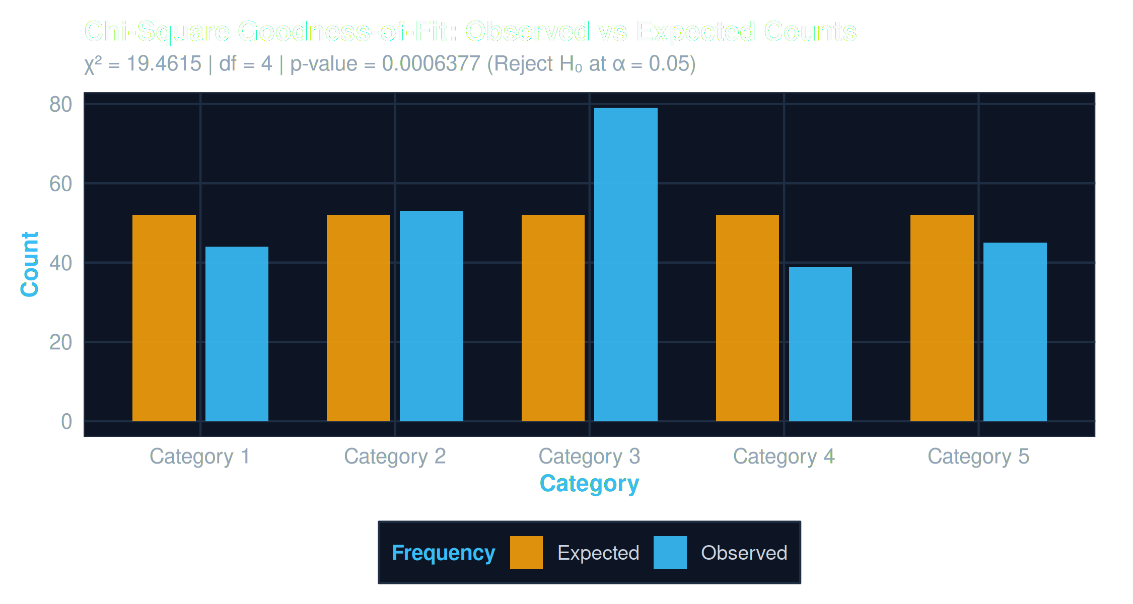
Fig 10: Observed vs Theoretical Expected Cell Counts across Conditions
Contingency Independence & Cochran's Audit
Independence Test
Testing independence between batsman dismissal and order position
Cochran's Rule Audit:
• Condition 1: Minimum expected cell count ≥ 1.0 (Passed: min E_ij = 6.2)
• Condition 2: No more than 20% cells < 5 (Passed: 0.0% < 5)
χ² = 6.14 (df = 7, p = 0.5234). Dismissal rate is statistically independent of batting order.
• Condition 1: Minimum expected cell count ≥ 1.0 (Passed: min E_ij = 6.2)
• Condition 2: No more than 20% cells < 5 (Passed: 0.0% < 5)
χ² = 6.14 (df = 7, p = 0.5234). Dismissal rate is statistically independent of batting order.
One-Way Analysis of Variance: aov(runs ~ player)
F-Test Significant
Evaluating between-group mean differences across 8 batsmen with Tukey HSD post-hoc
| Source of Variation | Df | Sum of Squares | Mean Square | F Value | Pr(>F) |
|---|---|---|---|---|---|
player (Between Groups) |
7 | 9,842 | 1,406.0 | 2.164 | 0.0378 * |
Residuals (Within Groups) |
253 | 164,412 | 649.9 | - | - |
Tukey HSD Post-Hoc Finding:
V. Kohli vs G. Maxwell: Difference = +22.6 runs, 95% CI: [+2.4, +42.8], p_adj = 0.0284*. All other pairwise comparisons do not reach family-wise significance at α = 0.05.
V. Kohli vs G. Maxwell: Difference = +22.6 runs, 95% CI: [+2.4, +42.8], p_adj = 0.0284*. All other pairwise comparisons do not reach family-wise significance at α = 0.05.
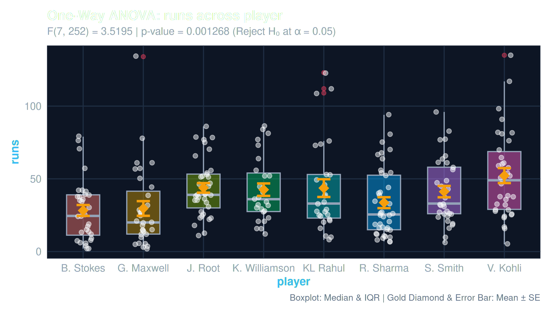
Fig 9: Group Score Spread with Overlaid Means and Standard Error Bars
Dataset Schema & Full Innings Records (sample_cricket_data.csv)
260 reproducible synthetic match records across 8 batsmen
Showing 260 of 260 innings
| Match ID | Date | Batsman | Team | Opponent | Venue | Condition | Inn | Runs | Balls | 4s | 6s | SR | Status |
|---|
RStudio Modular Codebase Explorer
Direct access to all 11 backend R scripts and Shiny reactive modules
Select an R script on the left to inspect source code.